• Group members
• Presentation
• Introduction
• Assignment description
• Experiment Results
• Conclusions, remarks or discussions
• Source code
• Answers to questions
• References

Christian Graf
Uli Schroeder
YongTao Zou

1. Introduction

   Approximate calculations of local displacement fields can be based on analyzing the optical flow, which is defined by the changes in image irradiances from image E_i to image E_i+1 of an image sequence. The optical flow can be analyzed for arbitrary image sequences. The optical flow is also, for example, of interest for calculating motion estimations in the area of active vision, or animate vision.

2. Assignment description

   Optical flow is defined by the changes in image irradiances from image E_i to image E_i+1 of an image sequence. The optical flow describes the direction and the speed of the object in the image.

   In general we consider the optical flow highly correlated to the local displacement but in reality it cannot be identified with it. For example consider a sphere showing no surface texture that is rotating in front of a camera. No optical flow can be observed even though a motion of object points occurs, i.e. the motions of surfaces showing no surface texture. On the other hand, for a static sphere and changing lighting conditions an optical flow can be observed for the sphere surface although no motion of surface points takes place. The optical flow can also depend on instability of the camera sensor, on changing illumination, or on different surface appearance for different viewing directions. Thus it is clear from the beginning the optical flow only allows to approximate local displacement fields in some cases. Ideally the optical flow is identically to the local displacement field.

   The basic Horn-Schunck methods uses this assumptions.

   Implementation (of the basic Horn-Schunck Algorithm)
   We have implemented our program to be run in a batch environment, so without interaction with the user. All parameters are given through the commandline:

   ./ass3horn [inputfile] [outputfile] [mode(1-3)] [number of iterations] [value of lambda] [initalU] [initialV]

   The input parameters and the input Results are checked to prevent the most likely crashs. The output is done directly on a HWindow which means that we could use its methods to draw circles and lines. To be able to draw the flow representation even for points at the border of the window, we defined an offset and factor which specify some extra space. An enlargement factor was introduce to make the lines more visible. As the window handling with Halcon is not that fast, we had to add a pause before being able to write to the canvas. Otherwise there would be some points in the upper left part missing.

   begin
     for j=: 1 to N do for i=:1 to M do begin:
        calculate the values Ex(i, j, t), Ey(i,j,t), and Et(i, j, t);
        {special cases for image points at the image border have to be taken into account}
        initialize the values u(i, j) and v(v, j) with zero
     end {for};
     choose a suitable weighting value lambda {e.g. lambda=0.1)
     choose a suitable number n0>=1 of iterations; {n0=8}
     n:=1;
     while n<=n0 do begin
     for j:= 1 to N do for i:=1 to M do begin
        udash=(u(i-1,j) +u(i+1, j) + u(i, j-a) +u(i, j+1))/4;
        vdash=(v(i-1,j) +v(i+1, j) + v(i, j-a) +v(i, j+1))/4;
        {leave image points at the image border unconsidered}
        alpha=Ex(i,j,t)*udash+Ey(i,j,t)*vdash +Et(i, j, t)*lambda/(1+lambda(Ex(i, j, t)^2 +Ey(i, j, t)^2);
        u(i, j)=udash -alpha* Ex(i,j,t);
        v(i, j)=vdash-alpha*Ey(i, j, t)
     end{for};
     n=n+1;
     end{while}
   end;

   The local differences are computed with a simple and an advanced one. The first one simply computes the difference between the current and next pixel value E(i,j) - E(i,j+1). The advanced one is the method used by Horn-Schunk. For each run we calcullate and store the least square error of u and v for the iteration step. Thus we can see how fast they converge against zero with the given parameter. This is one of the criterias we used for our evaluation.

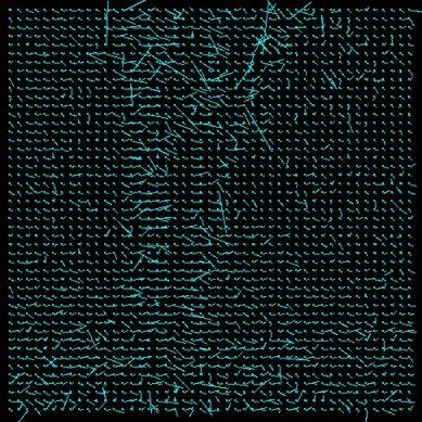
   Representation
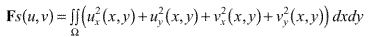
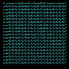
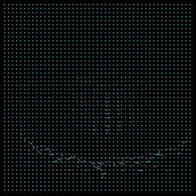
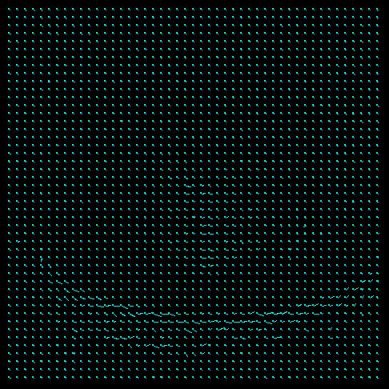
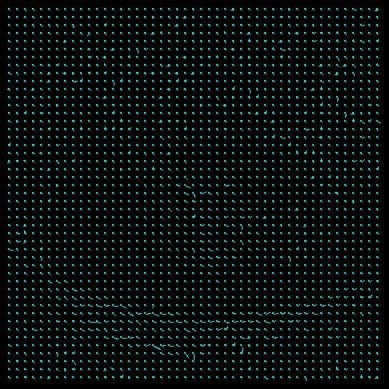
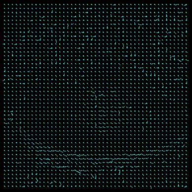
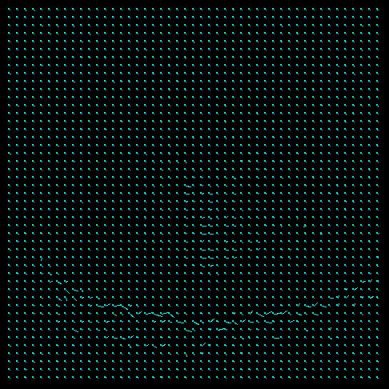
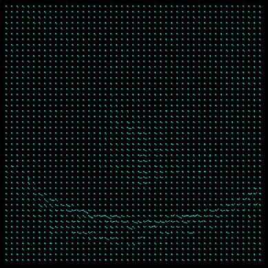
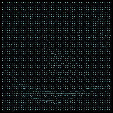
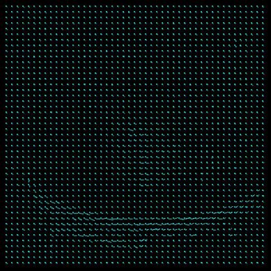
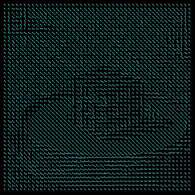
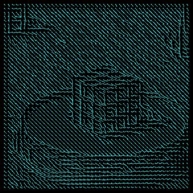
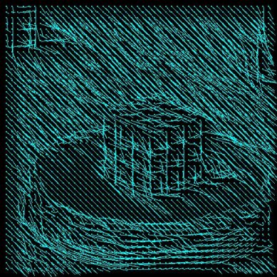
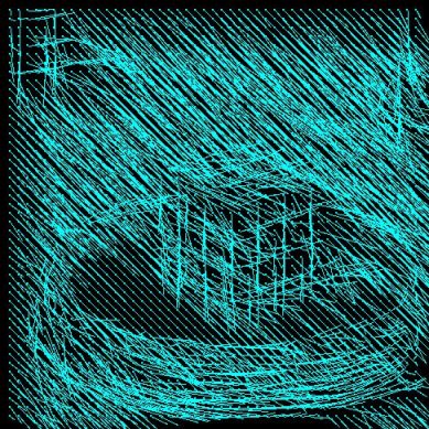
   A needle map is used to represent the Results. Not every point is drawn with its correspondent representation of the displacement (basically a line), but only some of them. Those are regularly chosen from the original dataset by applying a grid an the image. The grid width once was 10 points but was refined to 5 because with just a few data samples the flow in the Results is not clearly visible (loss of information). From testing it has shown that too many needles in the image only confuse and hide information. For getting clearer representation we deciced to enlarge the needles by a factor of 3.

3. Experiment Results

   We could't present the whole range of possible Results on the original due date and thus no findings about Horn-Schunck because we were constantly handicapped by the computer system of the University. We refuse any responsibility for that and the inability to hand-in materials and draw our conclusions in time.

   Camparison of methods for local differences with different Results
   iterations=8 lambda=0.1 u(i,j)=v(i,j)=0
   

   simple forward	advanced forward
   sqare
   LSE_u: 0.0011307    LSE_v: 0.0013669	LSE_u: 0.0017220    LSE_v: 0.0016719
   mysine
   LSE_u: 0.0001125    LSE_v: 0.0000332	LSE_u: 0.0000908    LSE_v: 0.0000408
   rubic
   LSE_u: 0.0003402    LSE_v: 0.0001016	LSE_u: 0.0000844    LSE_v: 0.0000827
   trees
   LSE_u: 0.0002889    LSE_v: 0.0008819	LSE_u: 0.0006038    LSE_v: 0.0005663

   It can be easily observed that the Horn-Schunk method computes the flow more acurately. The needle map is clearer and has less errors and noise on it, but this depends on the image. Looking at the least square error (LSE) reveals an arbitrary image: sometimes the LSE correspond with the visuable Results (advanced forward method should have a less LSE after the iterations than the simple forward method), sometimes not.
   The Horn-Schunk needs more compution time (if this is relevant) but anyhow we chose it as the appropiate method for all further tests. From the observation of this experiment we chose the rubic?.jpg as Results for the further tests, because it seems to have a good noise-data relation which Results in a clear Horn-Schunk representation. Some other parameter seem not to be chosen that well (enlargement factor), because there are artefacts and obviously errors in the needle map (to long lines...).

   Camparison of different lambda values
   iterations=8 u(i,j)=v(i,j)=0
   

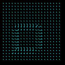
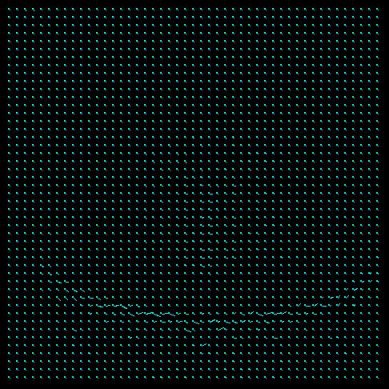
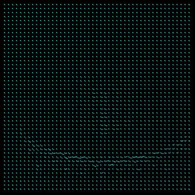
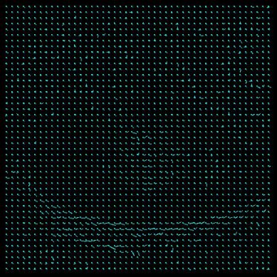
   lambda=0.001 LSE_u: 0.0000638    LSE_v: 0.0000101	lambda=0.01 LSE_u: 0.0000653    LSE_v: 0.0000164
   lambda=0.1 LSE_u: 0.0000908    LSE_v: 0.0000408	lambda=1.0 LSE_u: 0.0001273    LSE_v: 0.0000978
   lambda=10 LSE_u: 0.0001377    LSE_v: 0.0001055	lambda=100 LSE_u: 0.0001391    LSE_v: 0.0001062

   With this Results we can see that for high values of lambda the Results become noisy but the Horn-Schunk effect a little clearer. But this effect get vanished in the noise. So we decided to take a good noise/Horn-Schunk effect relation which seem to be given with lambda=0.1. The next step (lambda=1.0) includes noticable noise but in the image before (lambda=0.01) the Horn-Schunck effect is too subtle. The comparison of the LSE in the different runs shows that the higher the lambda the less is the LSE converging against zero. So a relatively small lambda is more effective. Thus we used lamda=0.1 as default in the whole test.

   Camparison of different iteration steps
   lambda=0.1 u(i,j)=v(i,j)=0
   

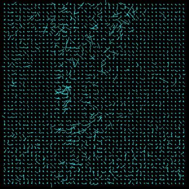
   iterations=1 LSE_u: 0.0229580    LSE_v: 0.0079244	iterations=2 LSE_u: 0.0017817    LSE_v: 0.0009416
   iterations=5 LSE_u: 0.0002067    LSE_v: 0.0000927	iterations=8 LSE_u: 0.0000908    LSE_v: 0.0000408
   iterations=10 LSE_u: 0.0000612    LSE_v: 0.0000280	iterations=20 LSE_u: 0.0000168    LSE_v: 0.0000084

   With more iterations the Horn-Schunck effect gets clearer and more accurate. A comparison between the first and the last Results definetly shows that (and the comparison of the LSE proves it). Concerning the computation time, the more iterations the more time is spend and the more memory allocated. Surprisingly the case with ten iterations shows heavy noise in some part. We think that with eight iterations the Results is sufficiently clear and thus used this value as default for all tests.

   Camparison of different initial values for u and v
   iterations=8 lambda=0.1
   

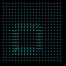
   u(i,j)=v(i,j)=0	u(i,j)=v(i,j)=1
   u(i,j)=v(i,j)=2	u(i,j)=v(i,j)=5
   u(i,j)=v(i,j)=10

   The initial value of u and v influence the algorithm in the wat that they predetermine of certain direction of the flow tensors (represented as strokes). In our experiment we can observe that a from different u,v there are largely different outputs. Some might be interesting from the view point of an artist, but for the exact representation of the Horn-Schunck solution they seem not suitable. That mostly because the artist like style of the output is noise (artificially inserted) in the image processing sense.

4. Conclusions, remarks or discussions

   This assignment almost exclusively considers motions of scene object as causes of scene changes.Optical flow is defined by the changes in image irradiances from image E_i to E_i+1 of an image sequence. We use Horn-Schunck method in this assignment. All image points is treated equally, independent from the (unknown) distance of the projected object surface points to the image plane.

   We would appreciate if the computer system in the university was permanently working and not be in a constant 'pre-release' phase!

5. Source code

   Source for the Horn-Schunck operator

1. What assumptions have you made?

   In general:
   1	Constant time difference between capturing of two pictures of the image sequence.
   2	constant irradiance values The change of brightness is entirly caused by absolute object motions, not by camera or light motion. The whole scene is stable over time.
   3	image value fidelity Points from the one image appear in the second Results at other positions but with the same brightness value.
   4	The optical flow is uniquely defined (actually different optical flow models may specify different vector fields). Let ui(x,y)=(ui(x,y),vi(x,y)) be the optical flow from image Ei to Ei+1, which characterizes the change from image Ei to Ei+1.
   5	motion fidelity The high correlation between optical flow and local displacement is expected. An error between the ideal and the actual correlation can be used to define an error measurement for evaluating the calculated optical flow as well as being an additional assumption for the derivation.
   For the implementation of the Horn-Schunck algorithm:
   6	The image function E(x,y,ti) can locally be represented by a Taylor expansion for a small step (delta_x,delta_y,delta_t).
   7	Image brightness E(x,y,t) is a continuous and differentiable function of three variable x, y and t.
   8	The higher order terms of the Taylor expansion of E(x, y, t) are zero (e=0).

2. What is the Horn-Schunk constraint?

The Taylor expansion of E(x,y,t_i) for a particular step (u_i(x,z), V_i(x,y),delta_t_const) is considered. The Horn-Schunck constraint follows from the assumed image value fidelity of the optical flow, and from the assumption that these optical flow vectors only describe small steps for which the linearity assumption for E(x, y, ti) is satisfied, i.e. for which e=0 can be assumed.

The Horn-Schunck constraints can also be derived assuming the more appropriate motion fidelity constraint of the optical flow. For the Taylor expansion of the image function it is assumed at first that the error term e is approximately in the order of aberration.

The time scale factor delta_t=const=1 is used in the following for formal simplification. In the following the values t_i=i, for i=0,1,2,... or t=0,1,2... specify the discrete times at which the individual pictures of image sequence are taken.

The Horn-Schunck constraint restricts the possible value range of the optical flow onto a straight line in the uv-space. The intersections of this line with the u-axis or the v-axis are equal to (-Et/Ex, 0) or (0, -Et/Ey), respectively. The vector (Ex, Ey) is perpendicular to the straight line.

3. What do Fs and Fh represent?

Fs indicates the smoothness error for a function pair (u(x,y), v(x,y)). It constrains that variation of the flow between neighbouring locations is small. Assume that nearby points within the image plane move in a similar manner. So the functional

has to be minimized which indicates the smoothness error.

Fh is error functional of Horn-Schunk constraint. It indicates that the observed intensity is constant for a constant location in camera/world space. Since the Horn-Schunck constraint has to be satisfied at the same time for all image points p=(x,y) of the given image sequence for a moment t, a solution for (u,v) for this time t also has to minimize the functional


4. What is the aperture problem?

Let us assume that an image edge passes through the image point (i,j). If the local displacement vector( i.e. the projection of the 3D motion) is orthogonal to the image edge in this point then the optical flow vector and the local displacement vector coincide( i.e. the motion fidelity is satisfied). But if, for instance, the local displacement vector runs in the same direction as the image edge, i.e. this vector is parallel to the image edge, then the null vector is calculated as an optical flow vector. This inaccuracy of the calculated optical flow (compared to the aspired local displacement vectors) is a concrete expression of the aperture problem. There is no general way to calculate the (unknown) local displacement vector from the calculated optical flow vector and the also calculable image value gradient. So the optical flow will always be only an approximation of the local displacement field. If the image value gradient is the null vector then the optical flow can also( approximately) be just the null vector.